Silicon strip detector calibration¶

This section contains description of the Silicon Strip Detector (SSD) calibration using ₂₂₆Ra alpha particle source.

Sections

Calibration algorithm ¶

General assumptions ¶

The main assumptions the method is based:

Detector and readout system responses are linear

\[E = aN + b,\]

where \(E\) - energy in [eV] dimensionality, \(N\) - readout value in ADC-channels count dimensionality, \(a\) and \(b\) - calibration coefficients;

Dead layer is uniform;
G4EmStandardPhysics description of \(\alpha\)-particle energy losses in silicon is sufficient;
All \(\alpha\)-particles are stopped in the detector.

Dead layer thickness estimation ¶

₂₂₆Ra \(\alpha\)-particles source enables to perform calibration measures with several energies. In the under discussion method three lines are used \(E_1 = 4.7844\) [MeV], \(E_2 = 6.0024\) [MeV], \(E_3 = 7.6869\) [MeV].

Ionization losses depend on particle start energy and dead layer thickness which it passes through.

For the set of three spectrum lines, an energy losses of lines dependence on dead layer thickness can be characterized by the following dimensionless expression

\[\eta(d) = \dfrac{N_3 - N_2}{N_3 - N_1},\]

where \(N_1, N_2, N_3\) - peak positions of spectrum lines in ADC-channel counts, coincident with \(E_1, E_2, E_3\) energies in [MeV], and in linear calibration assumption it equals

\[\eta(d) = \dfrac{E_3 - E_2}{E_3 - E_1},\]

The figure 1 shows \(\eta(d)\) dependence (in silicon equivalent of thickness) calculated using Geant4 G4EmCalculator class and program LISE++.

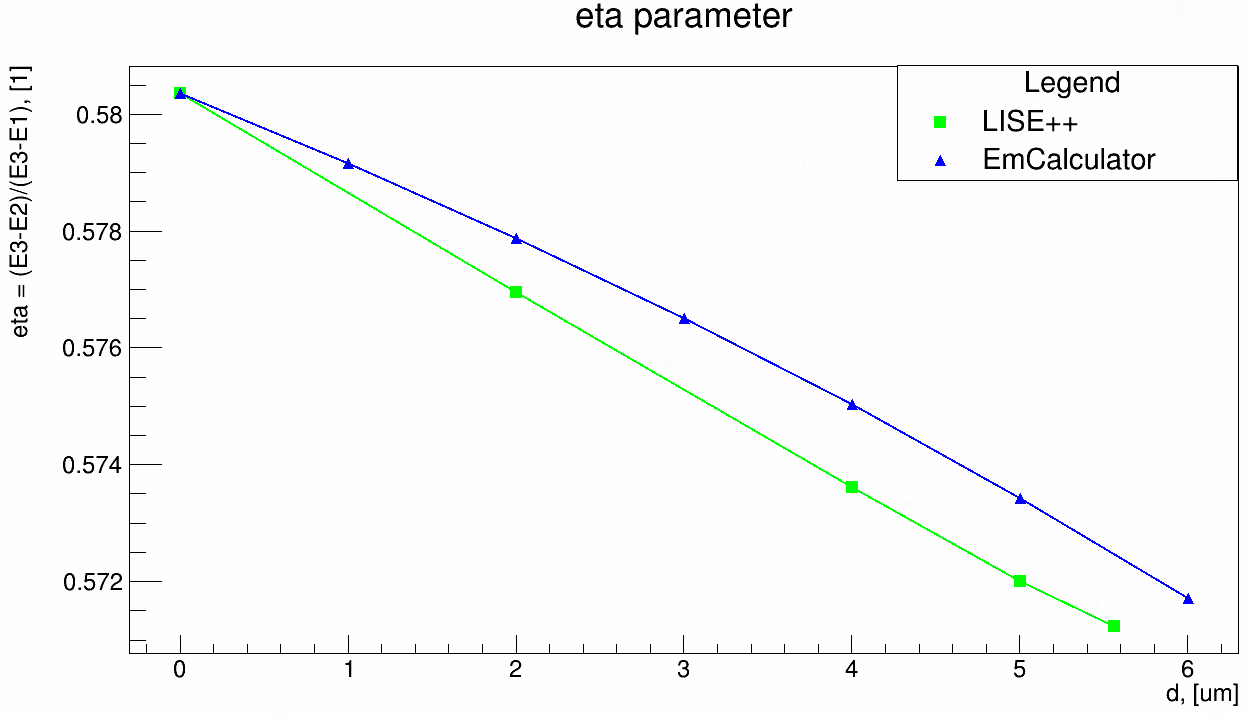
Figure 1. Dependence \(d(\eta)\), calculated using G4EmCalculator and LISE++

For the calibration procedure the quadratic approximation of the \(d(\eta)\) dependence shown in the figure 2 is used.

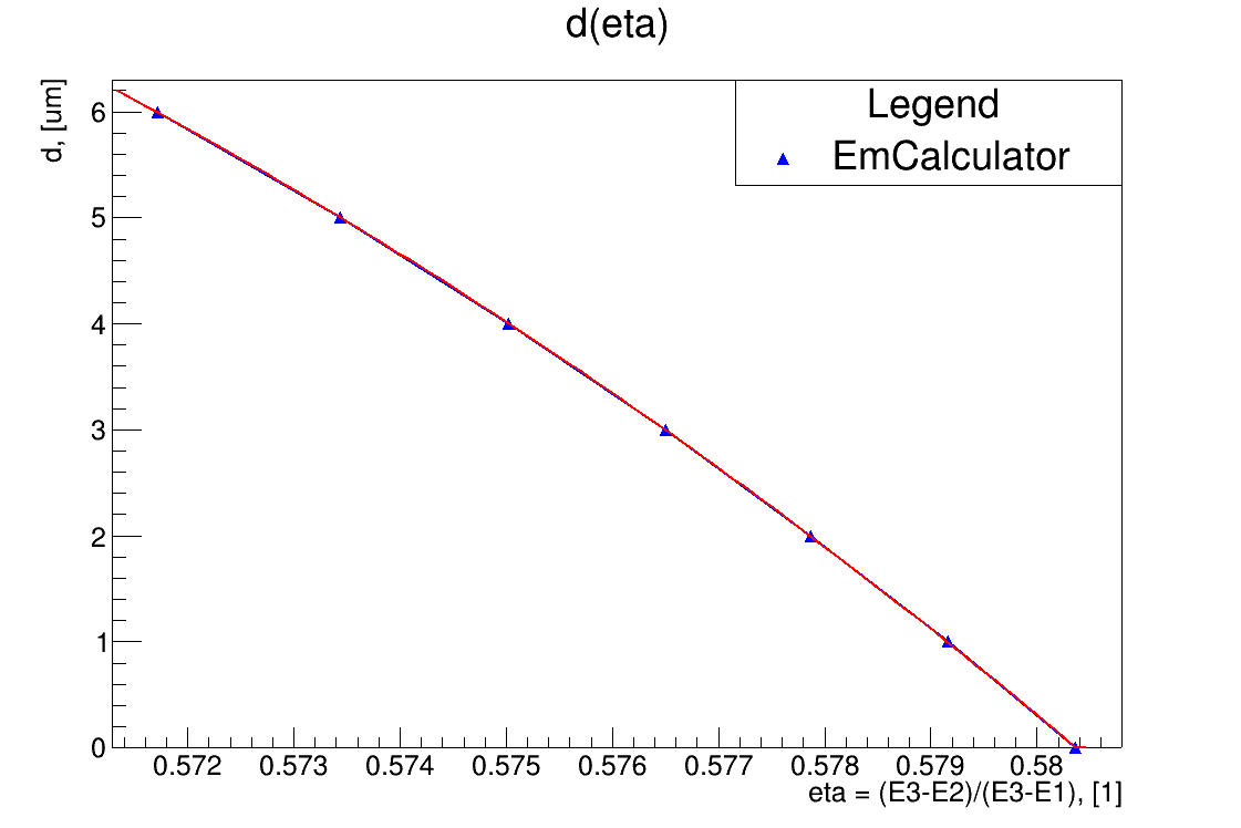
Figure 2. Quadratic approximation of the \(d(\eta)\) dependence

Approximation coefficients are listed in the table 1.

Table 1. Coefficients of the quadratic approximation \(d(\eta)=p_2 \eta^2 + p_1 \eta + p_0\)

\(p_2\)	\(p_1\)	\(p_0\)
17102.8129	19011.5041	-5272.9763

The typical form of the spectrum is shown in the figure 3.

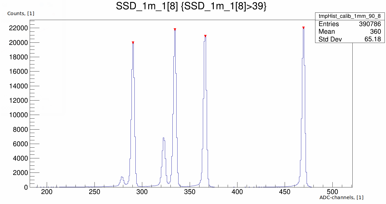
Figure 3. Typical spectrum. Red markers - peaks positions found by TSpectum algorithm

Algorithms of peaks positions determination are described in the section _set-peak-search-algorithm-type. The methodology of algorithm stability exploration is described in the section calibration-stability-research.

An accuracy of peak centroid position (RMS) determination by the ‘sliding window’ algorithm is about 0.05 ADC sampling step. In case of a large peak width accuracy goes downward.

The inaccuracy of the dead layer estimation concerned with the peak searching algorithm inaccuracy is 0.24 [\(\mu m\)] in case of the dead layer thickness about 2 [\(\mu m\)]. The assumption about strips-wise dead layer uniformity enables to treat each strip dead layer as averaged over the whole sensor. The averaging leads to accuracy in dead layer determination up to 0.06 \(\mu m\) (RMS).

The dead layer thickness found in such a way also includes the dead layer of the source cover ~0.3 [\(\mu m\)].

In the case of a thin detector (about 20 \(\mu m\)), the full stop of alpha-lines is occurred when the sensor is rotated for a significant angle (65 degrees) with respect to direct source exposure. An evaluated effective thickness must be re-calculated into real one according to angle.

Calibration coefficients determining ¶

The estimated dead layer thickness enables to evaluate energy deposit of \(\alpha\)-particles with different energies and calculate corrected readout energy value. Then three points \(E(N)\) are approximated by a straight line (figure 4).

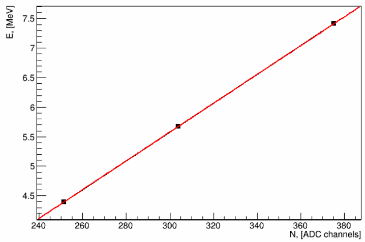
Figure 4. Calibration points linear approximation

Program realization ¶

The realization of algorithms is implemented as ROOT-macro. The input data is a file with raw data in a *.root format, produced by FLNR *.lmd life conversion library based on TNeEvent class using the Go4 system developed in GSI.

All the classes are described in the source code Doxygen documentation.

Calibration tools may be included to a user macro by the following:

#include "ERCalibrationSSD.cxx"

using namespace ERCalibrationSSD;

Class diagram ¶

The class diagram (figure 6) briefly presents relations between main program entities.

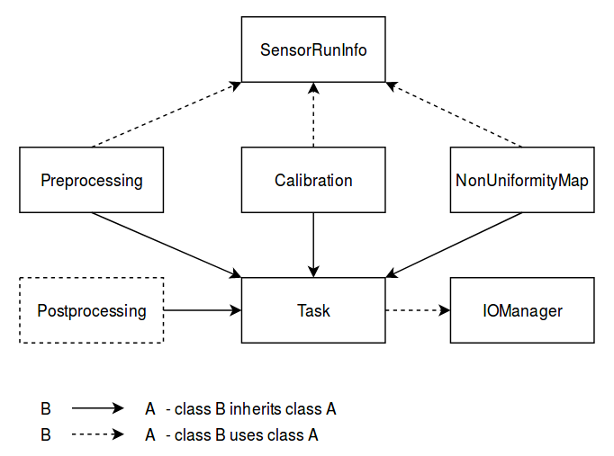
Figure 6. Class diagram

Task class is the base for all processing methods and aggregates

run_id which is istantiated by a base of a raw input file name.
CalibIOManager class instance which is responsible for a unified access to resulting files. It deploys the folder structure for results

result
├── [run_id]
│   ├── input - preprocessing resulting data.
│   └── [sensor_name]
│       ├── txt - text format results, thesholds, peaks position, etc.
│       ├── draw - ROOT format of results.
│       └── report_[run_id]_[sensor_name].txt
└── [run_id]
    ├── input - preprocessing resulting data.
    ├── [sensor_name_thin_sensor_name_thick] - files related to thin sensor thickness map building
    ├── [sensor_name_thin] - thin sensor data
    └── [sensor_name_thick] - thick sensor data

SensorRunInfo class stores information about path to the raw data, station name and histogram parameters during the processing.

Preprocessing ¶

The preprocessing is intended to clear input data for the calibration (or thin sensor thickness map) by leaving only analyzed stations leaves in a ROOT tree and preview of histograms for choosing calibration algorithm parameters.

auto prep_ssd_1m_1 = new Preprocessing(file_calib_path);
// several sensors may be added
prep_ssd_1m_1->AddSensor(ssd_1m_1);
prep_ssd_1m_1->ConvertTree();
prep_ssd_1m_1->FindThresholds();
prep_ssd_1m_1->MultiplicitySelection();

Using methods ConvertTree(), FindThresholds() and MultiplicitySelection() one can control intermediary results (thresholds finding quality), but commands can be executed by the command

prep_ssd_1m_1->Exec();

Solver ¶

Calibration procedure is prosecced by Calibration class and includes the following steps.

Peaks position determination.
Dead layer estimation.
Calibration coefficients calculation.
Report file printing.

Class constructor in the current reazalion keep path to a raw data file as a parameter.

auto calib_ssd_1m_1 = new Calibration(file_calib_path);

The report file is stored by path ./result/[run_id]/[sensor_name]/report_[run_id]_[sensor_name].txt.

Set peak search algorithm type ¶

Two peak search algorithms are implemented:

‘Sliding window’ (default) - a window of fixed width is slides left-to-right in the bounded region around peaks found by TSpectrum algorithm.
‘Gauss’ - fit bu Gauss with pol1 in fixed region around peaks found by TSpectrum algorithm.

Proper algorithm is set by SetPeakSearchMethod() method. Algorithm options and realization details may be found in Doxygen documentation.

calib_ssd_1m_1->SetPeakSearchMethod("sliding_window");
// TSpectrum parameters
calib_ssd_1m_1->SetFitMinSigma(6.);
calib_ssd_1m_1->SetFitPeakThreshold(0.7);
// 'Sliding window' parameters
calib_ssd_1m_1->SetSlideWindowWidth(10);
calib_ssd_1m_1->SetSearchRadius(15);

or

calib_ssd_1m_1->SetPeakSearchMethod("gauss");
// TSpectrum parameters
calib_ssd_1m_1->SetFitMinSigma(6.);
calib_ssd_1m_1->SetFitPeakThreshold(0.7);
// Gaus + pol1 parameter
calib_ssd_1m_1->SetSearchRadius(15);

Postprocessing ¶

For now, the postprocessing is not implemented as a special utility. User can validate results by viewing the report file and the calibrated spectra.

Data processing flow ¶

The full processing flow of calibration run data from readout to reconstruction verification is shown in the figure 7.

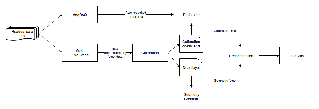
Figure 7. Data processing flow

AqqDAQ files for raw data conversion are available by link ACCULINNA_go4_user_library.
Full calibration run example ExpertRoot SSD calibration.
Digibuilding, reconstruction and analysis example ExpertRoot SSD reconstruction

LMD data conversion ¶

TNeEvent library ¶

TNeEvent is nominal name for a event library prepared for a certain experiment run. Library files libGo4UserAnalysis.rootmap and libGo4UserAnalysis.so should be in folder invoking Go4 library execution.

Before conversion, environment variables must be initialized by the execution of the go4login script from the Go4 library install location.

bash /path/go4login

All the *lmd files from dir_in may be converted to *.root files to dir_out by the following bash-script.

dir_in=/path/to/input/dir/
dir_out=/path/to/output/dir/
for file in dir*
do
fbname=$(basename "$file" .lmd)
if [ -f "$file" ]
then
go4analysis -file $file -store "{$dir_out}{$fbname}.root"
fi
done

AqqDAQ + Digibuilder ¶

The first step is repacking *lmd data to *root by AqqDAQ utilities. All the instructions on ACCULINNA_go4_user_library.

The Digibuilder is set of ExpertRoot classes. Example of it’s usage in the context of event reconstruction in thin sensor map building run may be found by the link.

Thickness map of the thin sensor ¶

A thin sensor effective thickness is not uniform. It can be defined using data from the measurement with simultaneous radiation exposure of an assembly of a thick sensor and a thin in the front of it shown in Figure 8.

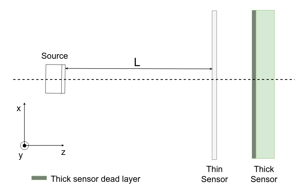
Figure 8. Thin and thick sensors radiation exposure

In such measurement only the high energy line comes throught thin sensor and registered in thick, so it is used for calibration.

An energy deposit in the thin station with respect to linear calibration assumption for each pixel (data registered on cross of two strips: one from thin station and another from thin) may be estimated by expression:

\[\Delta E = a(N_2 - N_1),\]

\(N_2\) and \(N_1\) - readout value from run with thick and thin sensors and with thick only respectively, \(a\) - calibration coefficient.

The full effective thickness including both thin sensor and dead layer depending on energy deposit is evaluated by qubic shown in figure 9.

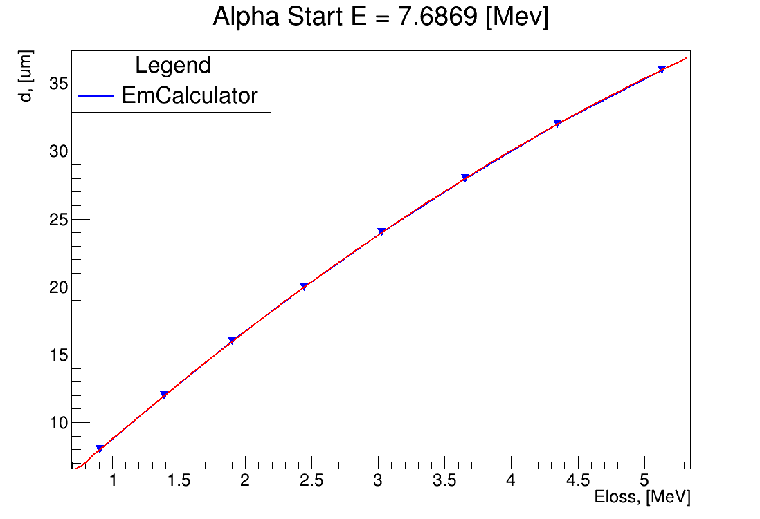
Figure 9. Qubic approximation of d(Delta E)

The fit coefficients are listed in table 2.

Table 2. Coefficients of the quadratic approximation \(d(\Delta E)=p_3 \Delta E^3 + p_2 \Delta E^2 + p_1 \Delta E + p_0\)

\(p_3\)	\(p_2\)	\(p_1\)	\(p_0\)
-0.0044059	0.00805579	9.18781	-0.401229

The last step is subtracting of the thick sensor dead layer:

\[d_thin = d_full - d_dead,\]

where d_thin - thin sensor effective thickness, d_full - full thickness, d_dead - thick sensor dead layer thickness.

Code example. Thin sensor thickness map buildind ¶

The NonUniformityMapBuilder class inherits Task class and inplements thin sensor thickness distribution calculation. It handles information about two stations and needs preliminary steps: thick sensor calibration, map building run data preprocessing.

const TString calib_run_path = "/thick_calib_path/file.root";
const TString map_run_path = "/map_path/file.root";
// Define run parameters
auto ssd_1m_1_cal = new SensorRunInfo("SSD_1m_1", 16, 1024, calib_run_path);
auto ssd_1m_1_map = new SensorRunInfo("SSD_1m_1", 16, 1024, map_run_path);
auto ssd_20u_1_map = new SensorRunInfo("SSD_20u_1", 16, 1024, map_run_path);

auto thickness_map = new NonUniformityMapBuilder(map_run_path);
// Set sensors parameters
thickness_map->SetThickSensor(ssd_1m_1_map);
thickness_map->SetThinSensor(ssd_20u_1_map);
thickness_map->SetThickCalibSensor(ssd_1m_1_cal);
// Set peak search algorithm parameters
thickness_map->SetPeakSearchMethod("sliding_window");
thickness_map->SetFitMinSigma(6.);
thickness_map->SetFitPeakThreshold(0.7);
thickness_map->SetSlideWindowWidth(10);
thickness_map->SetSearchRadius(15);
// Run map builder
thickness_map->Exec();

Resulting files are stored in text format in a ./result/[run_id]/[map_sensors_id]/txt/map_[...].txt and ROOT histogram ./result/[run_id]/[map_sensors_id]/draw/map_[...].root. The histogram is shown in figure 10.

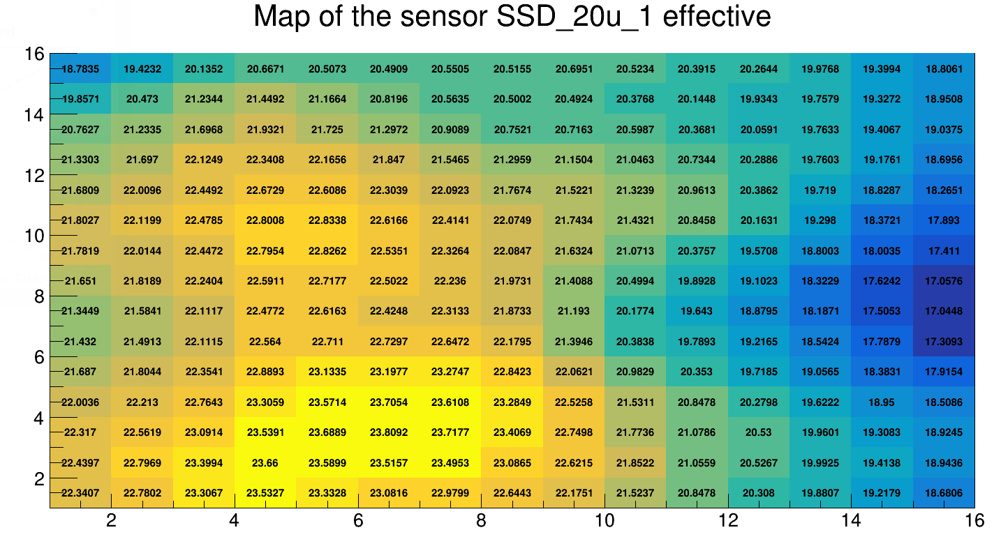
Figure 9. Thin sensor map ROOT file example

Verification ¶

Ionization models comparison ¶

The following tables demonstrate difference between energy losses estimations evaluated by LISE++ program and Geant4 G4EmCalulator class. Dependencies listed in tables 3-5 are fitted by quadratic line. The approximation example is shown in the figure 5 for 7.6869 [MeV] start energy.

Table 3. Start energy - 4.7844 [MeV]. \(dE(d)\) dependence evaluated by Geant G4EmCalculator and LISE++.

\(d\), [\(\mu m\)]	Geant4, [MeV]	LISE, [MeV]
2	0.302624	0.30463
4	0.617213	0.62423
6	0.947968	0.95791
8	1.296340	1.30900
12	2.059860	2.08110
16	2.960110	2.99460
20	4.130310	4.18250

Table 4. Start energy - 6.0024 [MeV]. \(dE(d)\) dependence evaluated by Geant G4EmCalculator and LISE++.

\(d\), [\(\mu m\)]	Geant4, [MeV]	LISE, [MeV]
2	0.260404	0.25998
4	0.527759	0.53050
6	0.804738	0.81157
8	1.091380	1.10100
12	1.697650	1.71350
16	2.362070	2.38580
20	3.104160	3.13770
24	3.968630	4.01680
28	5.057970	5.13250

Table 5. Start energy - 7.6869 [MeV]. \(dE(d)\) dependence evaluated by Geant G4EmCalculator and LISE++.

\(d\), [\(\mu m\)]	Geant4, [MeV]	LISE, [MeV]
2	0.219688	0.22259
4	0.443058	0.45036
6	0.671984	0.68333
8	0.906041	0.91841
12	1.390340	1.41010
16	1.901590	1.92640
20	2.443090	2.47640
24	3.023700	3.06320
28	3.651830	3.70330
32	4.344540	4.40770
36	5.131450	5.21050
40	6.068520	6.17800

Calibration stability research ¶

Stability in time ¶

The calibration stability in time was checked in long runs enabling divide full statistics into several files. Maximal standart deviations of calibration coefficients are shown in table 6 and demonstrate good stability.

Table 6. Maxumal standard devaitions of calibration coefficinets in time

Sensor	\(sigma_a\)	\(sigma_b\)
Thin	5.5e-5	0.016
Thick	6.5e-6	0.0059

On/off stability ¶

Turn-off the sensor and remeasurement shows significant inaccuracy in peak positions: up to 9 discrete steps. This result speaks that there good reasons to do calibrations without sensors turning off and opening the experimental camera.

Reconstruction ¶

Calibration parameters used in the reconstruction validation are listed in tables 7-8.

Table 7. SSD_1m_1 thick sensor calibration results

Strip number	a	b	\(d\), [\(\mu m\)]
0	0.0170136	-0.300991	2.14751
1	0.0169033	-0.377671	2.40688
2	0.0167126	-0.293483	2.48719
3	0.0165496	-0.378723	2.70073
4	0.016702	-0.38993	2.39342
5	0.0166474	-0.39643	2.67955
6	0.0168437	-0.35558	2.74014
7	0.016479	-0.273754	2.23416
8	0.0167534	-0.431799	2.53741
9	0.0169682	-0.269916	1.80624
10	0.0170281	-0.290404	2.32398
11	0.0171464	-0.28802	2.30622
12	0.0170073	-0.303184	2.28047
13	0.0171004	-0.268635	1.9785
14	0.0167947	-0.351776	2.44018
15	0.0164761	-0.350187	1.83882
		Avg.	2.33134

Table 8. SSD_20u_1 thin sensor calibration results.

Strip number	a	b	\(d\), [\(\mu m\)]
0	0.00508681	-0.11839	2.11252
1	0.00507884	-0.112467	2.10424
2	0.00520404	-0.116742	2.05644
3	0.00510507	-0.0809549	2.11519
4	0.00521461	-0.109044	1.98992
5	0.0051204	-0.0892601	2.10055
6	0.00511517	-0.109871	2.10648
7	0.00506191	-0.0841183	1.93686
8	0.00512354	-0.0867048	2.20535
9	0.00511479	-0.0644811	2.3923
10	0.00519145	-0.0966503	2.59457
11	0.00517657	-0.0799033	2.14259
12	0.00512621	-0.0975369	2.16496
13	0.0052136	-0.0672926	2.2285
14	0.00517104	-0.0885697	1.91963
15	0.00521849	-0.0544258	2.17915
		Avg.	2.14683

The source ₂₂₆Ra was set in 65 degrees with respect to the sensor’s normal so effective thickness (2.14 \(\mu m\)) should be recalculated to real (0.78 \(\mu m\)). In the front and backside of the sensor, the thickness is expected equal.

In independent exploration dead layer on source was estimated by value 0.3 \(\mu m\).

One sensor ¶

The reconstruction result for single thick detector is shown in figures 8-10. One can notice that difference from origin spectrum values (4.7844, 6.0024 and 7.6869 MeV) is less than 1 KeV.

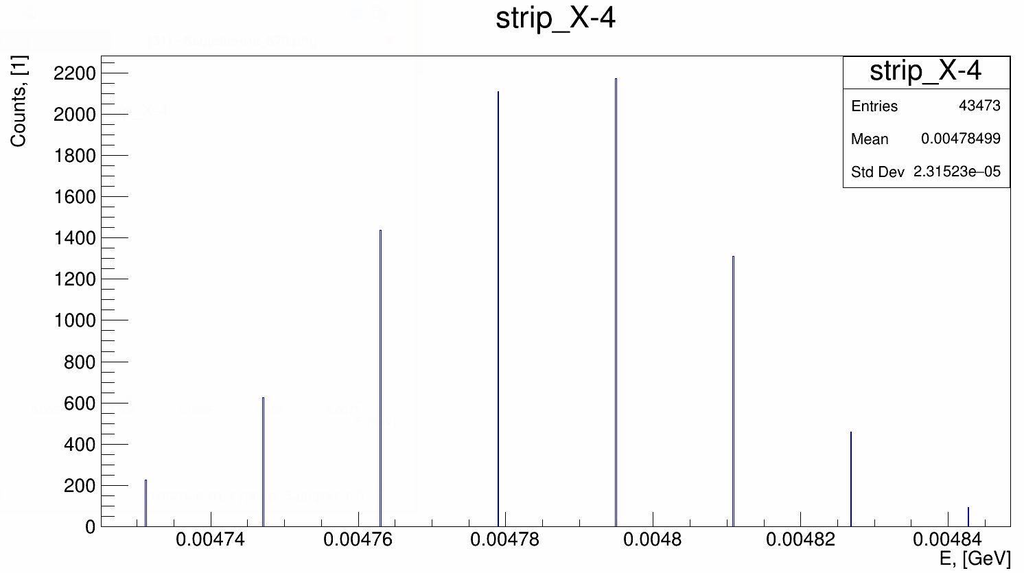
Figure 11. Reconstructed spectrum for the single thick sensor. Source passport energy 4.7844 MeV

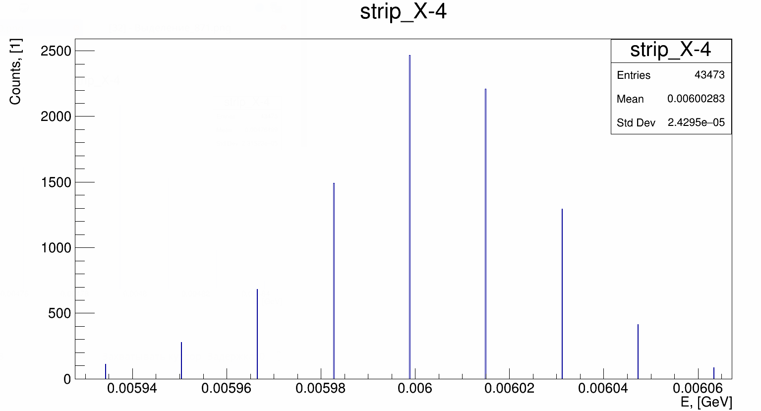
Figure 12. Reconstructed spectrum for the single thick sensor. Source passport energy 6.0024 MeV

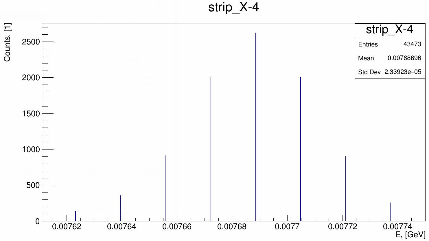
Figure 13. Reconstructed spectrum for the single thick sensor. Source passport energy 7.6869 MeV